The scSpecies workflow
This tutorial demonstrates how to apply the scSpecies workflow to align three scRNA-seq datasets (mice, humans and hamsters).
We start by loading the preprocesed .h5mu file saved within the data_prepocessing.ipynb notebook.
[1]:
import os
import muon as mu

mu.set_options(pull_on_update=False)

path = os.path.abspath('').replace('\\', '/')+'/'
mdata = mu.read_h5mu(path+'data/liver_atlas.h5mu')
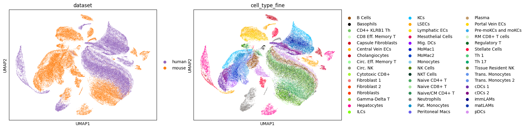
Before we pre-train scSpecies, we plot a UMAP representation of the unaligned mouse/human dataset pair on the data-level.
[4]:
from scipy import sparse
import anndata as ad
import scanpy as sc
import pandas as pd
import numpy as np

from scspecies.plot import return_palette
from scspecies.models import neighbors_workaround

# Subsetting to homologous genes
_, hom_ind_mouse, hom_ind_human = np.intersect1d(mdata.mod['mouse'].var_names, mdata.mod['human'].var['var_names_transl'], return_indices=True)

adata_concat = ad.AnnData(
    X=sparse.vstack([mdata.mod['mouse'][:, hom_ind_mouse].X, mdata.mod['human'][:, hom_ind_human].X]).toarray(),
    obs=pd.concat([mdata.mod['mouse'].obs, mdata.mod['human'].obs])
).copy()

# Color scheme for the liver cell dataset. Won't return nice results for other datasets.
palette = return_palette(list(adata_concat.obs.cell_type_fine.unique()) + list(adata_concat.obs.dataset.unique()))

sc.pp.pca(adata_concat)

# sc.pp.neighbors can crash the kernel for M1/M2 chips. We use a workaroung for this function.
#sc.pp.neighbors(adata_concat, use_rep='X_pca')
neighbors_workaround(adata_concat, use_rep='X_pca')

sc.tl.umap(adata_concat)
sc.pl.umap(adata_concat, color=['dataset', 'cell_type_fine'], palette=palette)
1) Context and target dataset alignment
scSpecies class.[ ]:
from scspecies.models import scSpecies
import torch

device = ("mps" if torch.backends.mps.is_available() and torch.backends.mps.is_built() else "cuda" if torch.cuda.is_available() else "cpu")

model = scSpecies(device,
                mdata,
                path,
                context_key = 'mouse',
                target_key = 'human',
                random_seed=1234
                )
Initializing context scVI model.
Initializing target scVI model.
train_context for 30 epochs and save the model parameters to path.get_representation an save them in the context modality in the .obsm layer.[15]:
model.train_context(30, save_key='_mouse')
model.get_representation(eval_model='context', save_intermediate=True, save_libsize=True)
Pretraining on the context dataset for 30 epochs (= 8820 iterations).
Progress: 99.9% - ETA: 0:00:00 - Epoch: 30 - Iteration: 8813 - ms/Iteration: 19.45 - nELBO: 1463.5 (+0.869) - nlog_likeli: 1445.1 (+0.879) - KL-Div z: 15.306 (-0.024) - KL-Div l: 3.0632 (+0.014).           Saved /Users/cschaech/Desktop/scpecies_package/scspecies/params/config_dict.pkl
Saved /Users/cschaech/Desktop/scpecies_package/scspecies/params/context_config__mouse.pkl
Saved /Users/cschaech/Desktop/scpecies_package/scspecies/params/context_optimizer__mouse.opt
Saved /Users/cschaech/Desktop/scpecies_package/scspecies/params/target_encoder_inner__mouse.pth.
Saved /Users/cschaech/Desktop/scpecies_package/scspecies/params/context_encoder_outer__mouse.pth.
Saved /Users/cschaech/Desktop/scpecies_package/scspecies/params/context_decoder__mouse.pth.
Saved /Users/cschaech/Desktop/scpecies_package/scspecies/params/context_lib_encoder__mouse.pth.
Calculate latent variables. Step 215/295
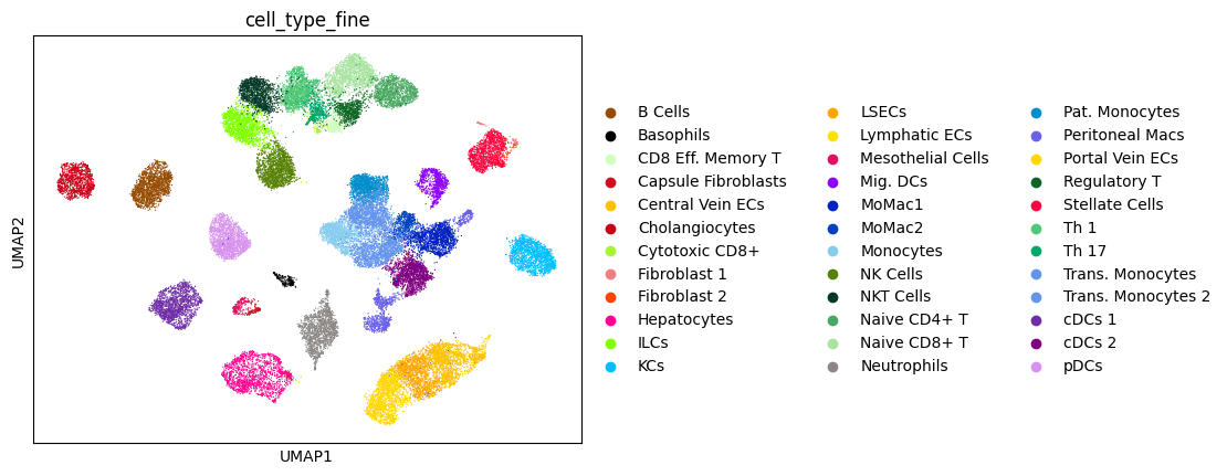
We check that the context scVI model has separated latent cell clusters by visualizing the latent representation with UMAP.
[16]:
#sc.pp.neighbors(model.mdata['mouse'], use_rep='z_mu')
neighbors_workaround(model.mdata['mouse'], use_rep='z_mu')
sc.tl.umap(model.mdata['mouse'])
sc.pl.umap(model.mdata['mouse'], color='cell_type_fine', palette=palette)
Next we fine-tune by training the target scVI model and aligning the human dataset with this latent representations.
[17]:
model.train_target(30, save_key='_human')
model.get_representation(eval_model='target', save_libsize=True)
Training on the target dataset for 30 epochs (= 8190 iterations).
Progress: 100% - ETA: 0:00:00 - Epoch: 30 - Iteration: 8190 - ms/Iteration: 38.69 - nELBO: 1874.3 (+3.259) - nlog_likeli: 1386.8 (+0.336) - KL-Div z: 13.879 (-0.002) - KL-Div l: 2.8306 (+0.003) - Align-Term: 470.84 (+2.922).            Saved /Users/cschaech/Desktop/scpecies_package/scspecies/params/config_dict.pkl
Saved /Users/cschaech/Desktop/scpecies_package/scspecies/params/target_config__human.pkl
Saved /Users/cschaech/Desktop/scpecies_package/scspecies/params/target_optimizer__human.opt
Saved /Users/cschaech/Desktop/scpecies_package/scspecies/params/target_encoder_inner__human.pth.
Saved /Users/cschaech/Desktop/scpecies_package/scspecies/params/target_encoder_outer__human.pth.
Saved /Users/cschaech/Desktop/scpecies_package/scspecies/params/target_decoder__human.pth.
Saved /Users/cschaech/Desktop/scpecies_package/scspecies/params/target_lib_encoder__human.pth.
Calculate latent variables. Step 213/274
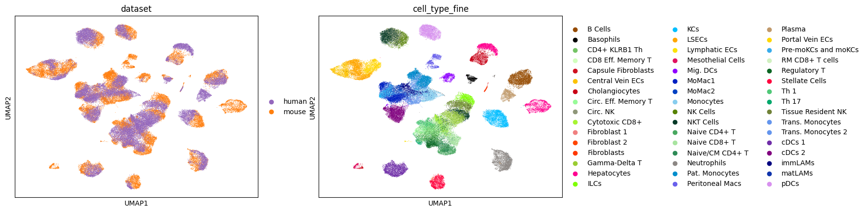
After fine-tuning, we can visualize the aligned latent representation.
[9]:
adata_concat.obsm['lat_rep'] = np.concat([mdata.mod['mouse'].obsm['z_mu'], mdata.mod['human'].obsm['z_mu']])

#sc.pp.neighbors(adata_concat, use_rep='lat_rep')
neighbors_workaround(adata_concat, use_rep='lat_rep')
sc.tl.umap(adata_concat)

sc.pl.umap(adata_concat, color=['dataset', 'cell_type_fine'], palette=palette)
2) Information transfer via similarity scores
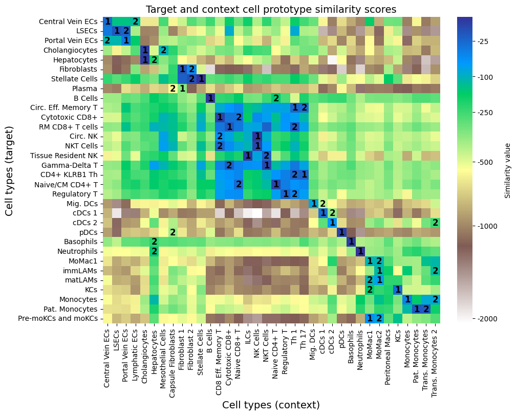
We continue by evaluating the likelihood based similarity measure between target and context cell types with return_similarity_df_prot.
scale=min_max or scale=max the scores are scaled such that the values can be interpreted as 1 = most similar. Without scaling the highest values (closest to zero) represent high similarity. The output dataframe contains target cell types in df.index and context cell types in df.columns.We can use these similarity scores to match cell type annotation between datasets. To reduce computational demand reduce the sample size via max_sample_targ and max_sample_cont.
[ ]:
from scspecies.plot import plot_prototype_sim_heatmap

import matplotlib.pyplot as plt
import seaborn as sns

df = model.return_similarity_df()
print(df.head())

plot_prototype_sim_heatmap(df)
1152/1152 Similarity calculation for the pDCs-pDCs pair                                                                           B Cells   Basophils  CD8 Eff. Memory T  \
B Cells            -3.801637 -293.414856        -207.617188
Basophils        -349.438416   -5.973221        -333.442078
CD4+ KLRB1 Th    -276.216736 -287.656647         -70.532181
Central Vein ECs -223.495178 -834.148071        -386.038269
Cholangiocytes   -391.894897 -720.851990        -314.666870

                  Capsule Fibroblasts  Central Vein ECs  Cholangiocytes  \
B Cells                   -228.771057       -362.112976     -239.511993
Basophils                 -246.749451       -340.687500     -247.973465
CD4+ KLRB1 Th             -193.275970       -376.608337     -239.761108
Central Vein ECs          -566.160706        -26.962593     -608.768433
Cholangiocytes            -198.600677       -368.269257       -6.315400

                  Cytotoxic CD8+  Fibroblast 1  Fibroblast 2  Hepatocytes  \
B Cells              -197.894989   -337.634277   -387.757141  -154.775330
Basophils            -327.910126   -266.688934   -279.753479  -198.024796
CD4+ KLRB1 Th         -61.268108   -229.415070   -303.099091  -148.981750
Central Vein ECs     -164.762054   -438.393799   -256.090271  -608.901733
Cholangiocytes       -299.564789   -319.764191   -385.411652  -467.067688

                  ...  Portal Vein ECs  Regulatory T  Stellate Cells  \
B Cells           ...      -270.722504   -241.138321     -249.516815
Basophils         ...      -271.414429   -321.340149     -267.381226
CD4+ KLRB1 Th     ...      -180.809570    -43.305161     -128.362900
Central Vein ECs  ...      -134.630371   -423.919281     -318.453003
Cholangiocytes    ...      -420.213501   -421.347961     -454.262207

                        Th 1       Th 17  Trans. Monocytes  \
B Cells          -465.809570 -186.778168       -248.952225
Basophils        -345.991516 -247.600815       -371.339966
CD4+ KLRB1 Th     -24.644609  -21.820202       -349.680908
Central Vein ECs -163.786545 -228.126785      -1017.947876
Cholangiocytes   -360.164917 -301.917175      -1015.759216

                  Trans. Monocytes 2      cDCs 1      cDCs 2        pDCs
B Cells                  -269.309326 -246.974823 -221.031967 -215.786346
Basophils                -391.958618 -404.020386 -329.501465 -391.551971
CD4+ KLRB1 Th            -381.546692 -373.724396 -325.895386 -294.512360
Central Vein ECs         -865.895569 -561.131836 -995.302246 -644.583984
Cholangiocytes           -775.300659 -398.324158 -833.397339 -449.033875

[5 rows x 36 columns]
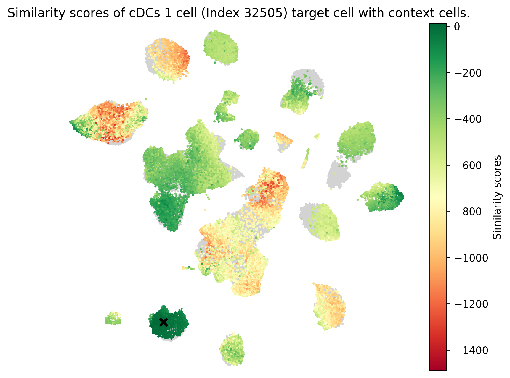
We can use the similarity measure to infer target label annotation from context cells.
transfer_labels_cell..obs labels specified in context_obs_transfer.df_neigbor dataframe contains all context cells with corresponding indices sorted by similarity.plot_similarity.[31]:
#from scspecies.plot import plot_similarity

human_cell_types = model.mdata['human'].obs['cell_type_fine']
mouse_cell_types = model.mdata['mouse'].obs['cell_type_fine']
common_cell_types = np.intersect1d(human_cell_types.unique(), mouse_cell_types.unique())

human_inds = human_cell_types.isin(common_cell_types).to_numpy().nonzero()[0]
human_ind = np.random.choice(human_inds)

context_obs_transfer = ['cell_type_coarse', 'cell_type_fine']
df_neigbor = model.transfer_labels_cell(human_ind, context_obs_transfer)

print('Index of target human cell: {}, Information: {}.'.format(str(human_ind), ', '.join([obs_name+': '+label for label, obs_name in zip(model.mdata['human'].obs[context_obs_transfer].iloc[human_ind].values[0], context_obs_transfer)])))
print(df_neigbor.head())

plot_similarity(adata_concat, df_neigbor, human_ind)
Index of target human cell: 32505, Information: cell_type_coarse: c, cell_type_fine: D.
                          cell_type_coarse cell_type_fine  index  \
AAAGCAACATATGAGA-41_mouse             cDCs         cDCs 1  18713
TCGAACAGTTGCATGT-12_mouse             cDCs         cDCs 1  17641
CGCTTCAGTATAATGG-41_mouse             cDCs         cDCs 1  18476
ACCATTTCATAATGAG-6_mouse              cDCs         cDCs 1  17809
CCACGGACAACGATGG-41_mouse             cDCs         cDCs 1  18415

                           similarity_score
AAAGCAACATATGAGA-41_mouse        -12.062500
TCGAACAGTTGCATGT-12_mouse        -11.791016
CGCTTCAGTATAATGG-41_mouse        -11.308228
ACCATTTCATAATGAG-6_mouse         -11.009521
CCACGGACAACGATGG-41_mouse        -10.935791
transfer_labels_dataset..obs layer of the target dataset.ret_pred_df.[20]:
context_obs_transfer = ['cell_type_coarse', 'cell_type_fine']
model.transfer_labels_data(context_obs_transfer)
print(model.mdata['human'].obs[['pred_sim_cell_type_coarse', 'cell_type_coarse', 'pred_sim_cell_type_fine', 'cell_type_fine']].head())
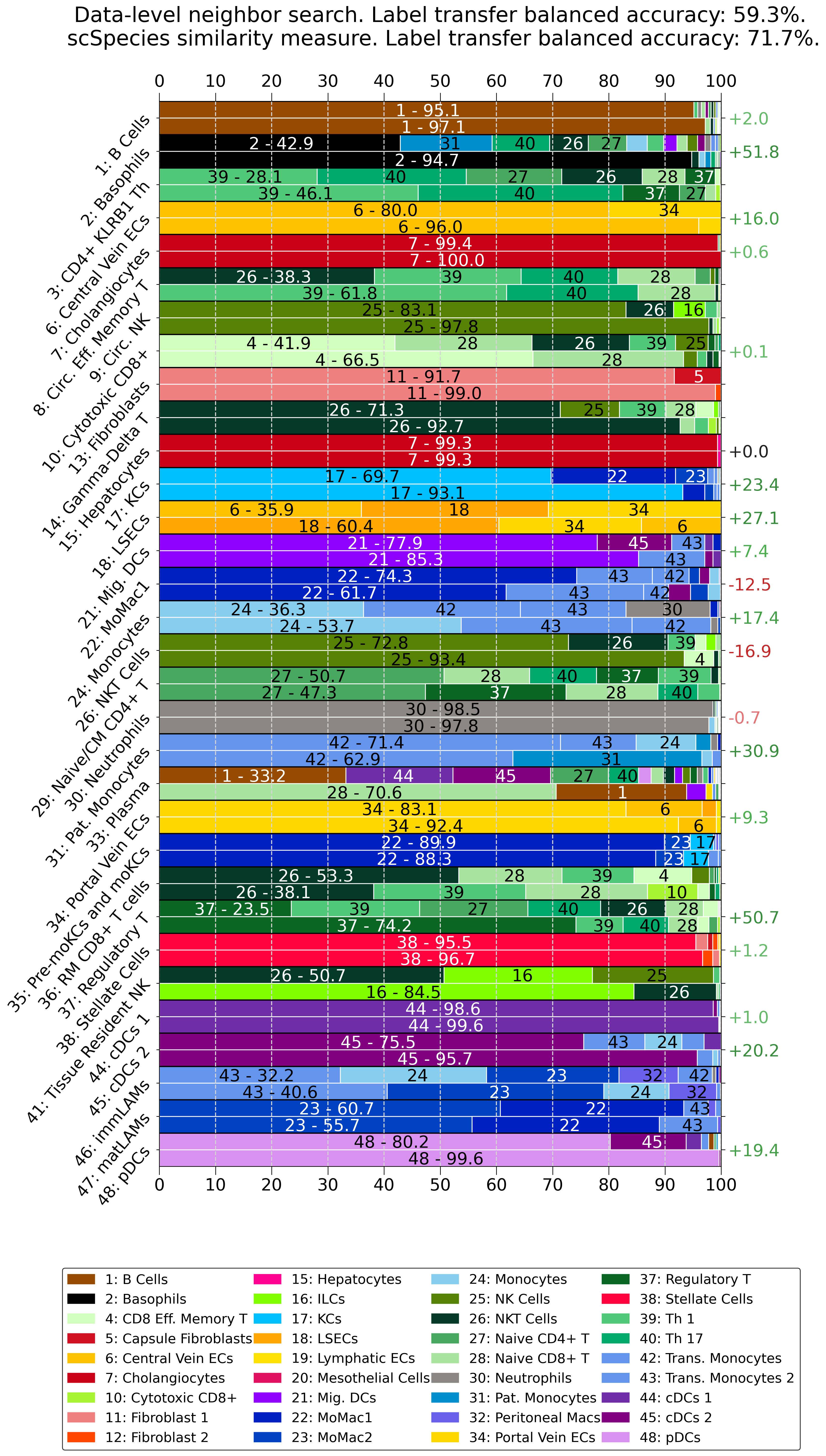
df_nns, bas_nns = model.ret_pred_df(pred_key='pred_nns_cell_type_fine', target_label_key='cell_type_fine', context_label_key='cell_type_fine')
df_sim, bas_sim = model.ret_pred_df(pred_key='pred_sim_cell_type_fine', target_label_key='cell_type_fine', context_label_key='cell_type_fine')
print(df_sim.head())
print('Data-level k=25 nearest neighbor search --> Balanced accuracy: {}%'.format(round(bas_nns*100,2)))
print('Label tarnsfer using similarity measure --> Balanced accuracy: {}%'.format(round(bas_sim*100,2)))
Pre-computing latent space NNS with 250 neighbors using the euclidean distance.
Calculate similarity metric. Step 273/274.                          pred_sim_cell_type_coarse   cell_type_coarse  \
TTCGGTCCACGGCCAT-12_human         Mono/Mono Derived  Mono/Mono Derived
TCATTTGCAGTCAGAG-1_human          Mono/Mono Derived  Mono/Mono Derived
TAGTTGGCATCCCACT-4_human          Mono/Mono Derived  Mono/Mono Derived
GGATTACTCCTCGCAT-12_human         Mono/Mono Derived  Mono/Mono Derived
TGGTAGTGTGGCTACC-28_human         Mono/Mono Derived  Mono/Mono Derived

                          pred_sim_cell_type_fine       cell_type_fine
TTCGGTCCACGGCCAT-12_human                  MoMac1  Pre-moKCs and moKCs
TCATTTGCAGTCAGAG-1_human                   MoMac1  Pre-moKCs and moKCs
TAGTTGGCATCCCACT-4_human                   MoMac1  Pre-moKCs and moKCs
GGATTACTCCTCGCAT-12_human                  MoMac1  Pre-moKCs and moKCs
TGGTAGTGTGGCTACC-28_human                  MoMac1  Pre-moKCs and moKCs
/Users/cschaech/Desktop/package_test/.venv/lib/python3.11/site-packages/sklearn/metrics/_classification.py:2480: UserWarning: y_pred contains classes not in y_true
  warnings.warn("y_pred contains classes not in y_true")
/Users/cschaech/Desktop/package_test/.venv/lib/python3.11/site-packages/sklearn/metrics/_classification.py:2480: UserWarning: y_pred contains classes not in y_true
  warnings.warn("y_pred contains classes not in y_true")
                    B Cells  Basophils  CD8 Eff. Memory T  \
B Cells           97.133333   0.000000           0.000000
Basophils          0.000000  94.736842           0.000000
CD4+ KLRB1 Th      0.000000   0.000000           0.066667
Central Vein ECs   0.000000   0.000000           0.000000
Cholangiocytes     0.000000   0.000000           0.000000

                  Capsule Fibroblasts  Central Vein ECs  Cholangiocytes  \
B Cells                           0.0               0.0             0.0
Basophils                         0.0               0.0             0.0
CD4+ KLRB1 Th                     0.0               0.0             0.0
Central Vein ECs                  0.0              96.0             0.0
Cholangiocytes                    0.0               0.0           100.0

                  Cytotoxic CD8+  Fibroblast 1  Fibroblast 2  Hepatocytes  \
B Cells                 0.266667           0.0           0.0          0.0
Basophils               0.000000           0.0           0.0          0.0
CD4+ KLRB1 Th           0.800000           0.0           0.0          0.0
Central Vein ECs        0.000000           0.0           0.0          0.0
Cholangiocytes          0.000000           0.0           0.0          0.0

                  ...  Portal Vein ECs  Regulatory T  Stellate Cells  \
B Cells           ...              0.0      0.000000             0.0
Basophils         ...              0.0      0.263158             0.0
CD4+ KLRB1 Th     ...              0.0     10.066667             0.0
Central Vein ECs  ...              4.0      0.000000             0.0
Cholangiocytes    ...              0.0      0.000000             0.0

                       Th 1      Th 17  Trans. Monocytes  Trans. Monocytes 2  \
B Cells            0.000000   0.066667          0.333333                 0.0
Basophils          0.000000   0.789474          0.000000                 0.0
CD4+ KLRB1 Th     46.066667  36.400000          0.000000                 0.0
Central Vein ECs   0.000000   0.000000          0.000000                 0.0
Cholangiocytes     0.000000   0.000000          0.000000                 0.0

                    cDCs 1    cDCs 2  pDCs
B Cells           0.000000  0.133333   0.0
Basophils         0.263158  0.000000   0.0
CD4+ KLRB1 Th     0.000000  0.000000   0.0
Central Vein ECs  0.000000  0.000000   0.0
Cholangiocytes    0.000000  0.000000   0.0

[5 rows x 36 columns]
Data-level k=25 nearest neighbor search --> Balanced accuracy: 59.25%
Label tarnsfer using similarity measure --> Balanced accuracy: 71.67%
[21]:
from scspecies.plot import label_transfer_acc

label_transfer_acc(df_nns, df_sim)
3) Differential gene expression analysis
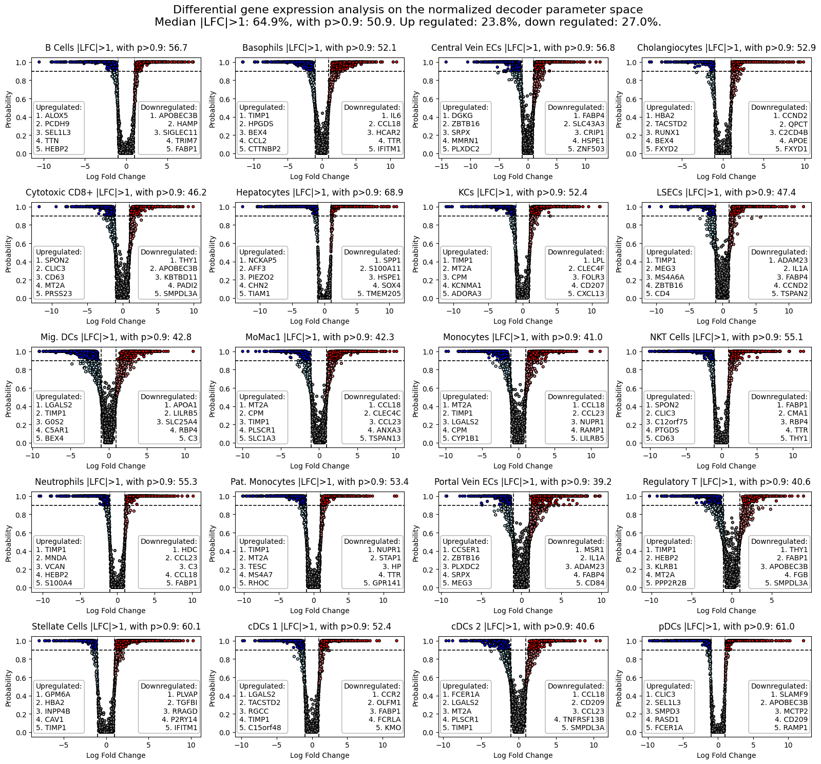
The difference in modeled gene expression can be analyzed by comparing the log2-fold change in normalized gene expression with compute_logfold_change.
[22]:
lfc_dict = model.compute_logfold_change(lfc_delta = 1)
The output is a dictionary with cell type wise data frames containing logfoldchange values and other information. The dataframes contain the homologous traget gene symbols in their index and their chosen labels as columns.
rho_median_context: Contains median context normalized gene expression,mu_median_context: Contains median context expected value gene expression,rho_median_target: Contains median target normalized gene expression,mu_median_target: Contains median target expected value gene expression,lfc: Contains mMedian Log2 fold-change of the relative expression parameter rho,p: Probability of Log2 fold-change values greater thanlfc_delta,lfc_rand: Contains median Log2 fold-change of the relative expression parameter rho on permuted data,p_rand: Probability of Log2 fold-change values greater thanlfc_deltaon permuted data.
[23]:
print('Results for', list(lfc_dict.keys())[0])
lfc_dict[list(lfc_dict.keys())[0]].head()
Results for B Cells
[23]:
| rho_median_context | mu_median_context | rho_median_target | mu_median_target | lfc | p | lfc_rand | p_rand | |
|---|---|---|---|---|---|---|---|---|
| C12orf75 | 5.061206e-08 | 0.000076 | 8.122530e-05 | 0.119411 | 6.281374 | 1.000000 | 3.767629 | 0.999940 |
| C1orf21 | 7.823262e-06 | 0.011871 | 4.618949e-06 | 0.007013 | -0.651978 | 0.118642 | -1.676469 | 0.972901 |
| C19orf33 | 2.573567e-05 | 0.038995 | 9.028594e-07 | 0.001343 | -3.805113 | 1.000000 | -5.364612 | 1.000000 |
| KIAA0513 | 1.432965e-05 | 0.022274 | 1.176323e-05 | 0.017654 | -0.283164 | 0.001989 | 0.007722 | 0.007634 |
| C15orf48 | 2.694451e-07 | 0.000411 | 5.526399e-06 | 0.008088 | 2.355554 | 1.000000 | 2.241066 | 1.000000 |
We can visualize the results with plot_lfc per cell type.
[24]:
from scspecies.plot import plot_lfc

plot_lfc(lfc_dict)
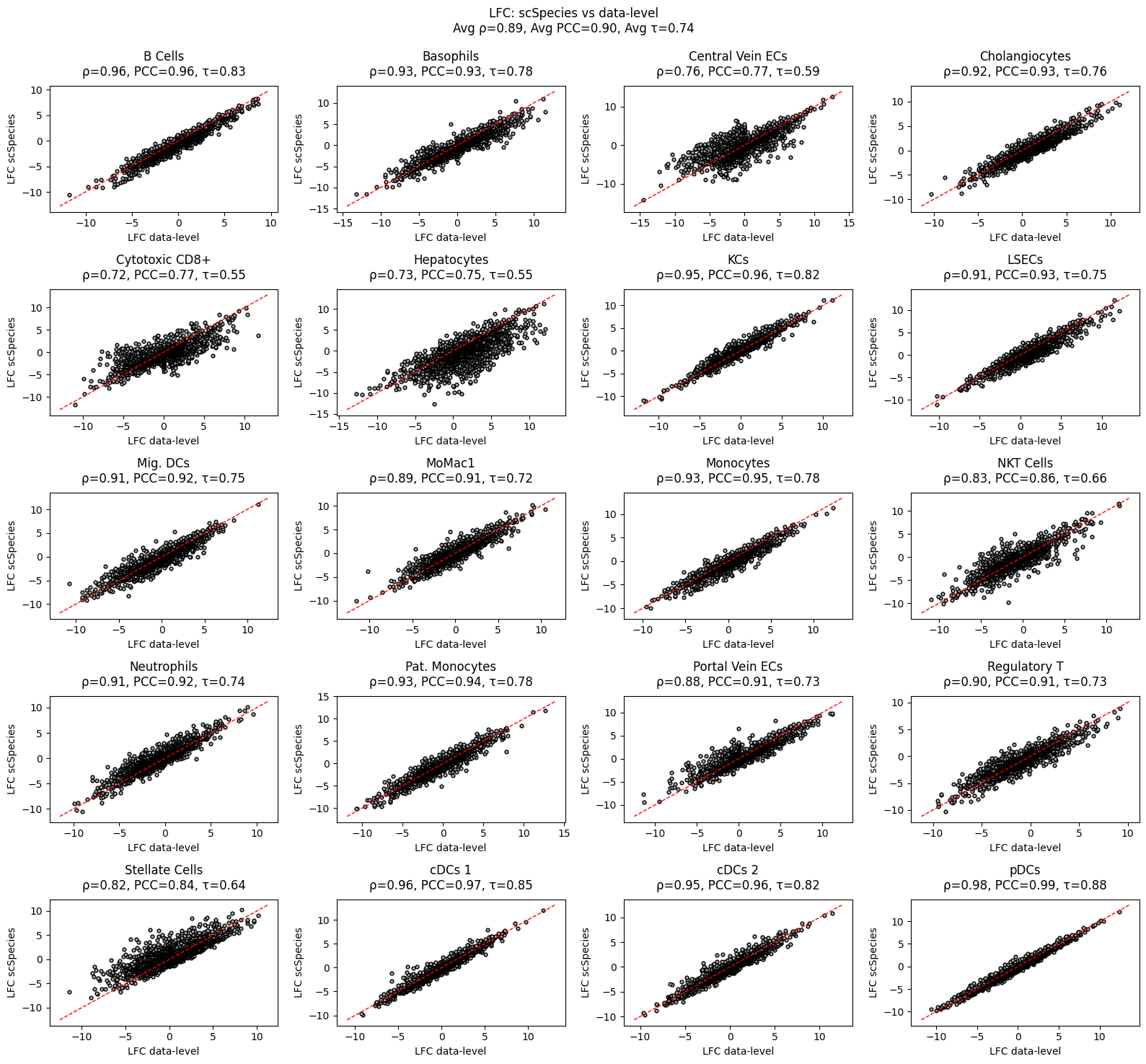
Lets compare the results with a DFG Analysis at the data level. For this we generate homologous cell samples from the latent space.
[25]:
from scspecies.plot import plot_lfc_comparison

target_rho_dict, context_rho_dict = model.generate_homologous_samples(samples=2000)
plot_lfc_comparison(model, lfc_dict)
.gmt file.[26]:
plot_cell_type = 'B Cells'
adata_h = ad.concat([ad.AnnData(target_rho_dict[key]) for key in target_rho_dict.keys()])
adata_h.var_names = model.mdata.mod['human'][:, model.target_config['homologous_genes']].var_names
adata_h.obs['cell_type_fine'] = np.concat([[key]*np.shape(target_rho_dict[key])[0] for key in target_rho_dict.keys()])
adata_h.obs_names_make_unique()
adata_m = ad.concat([ad.AnnData(context_rho_dict[key]) for key in context_rho_dict.keys()])
adata_m.var_names = adata_h.var_names
adata_m.obs['cell_type_fine'] = np.concat([[key]*np.shape(context_rho_dict[key])[0] for key in context_rho_dict.keys()])
adata_m.obs_names_make_unique()
#from scspecies.plot import load_and_filter_pathways
#gene_sets_path = '/Users/cschaech/Desktop/scSpecies/dataset/c2.all.v2024.1.Hs.symbols.gmt'
#pathways = load_and_filter_pathways(gene_sets_path, adata_h)
pathways = {'ABBUD_LIF_SIGNALING_1_DN': ['LIMS1','ITGA6','ENPP2','AHNAK','ALCAM','KLRB1','HK2'],
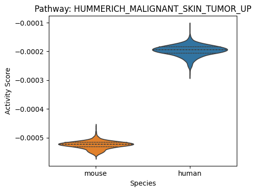
'HUMMERICH_MALIGNANT_SKIN_TUMOR_UP': ['S100A9', 'S100A8', 'LTF', 'CCND1', 'GSTO1','HBA2', 'COL18A1','SLPI','ECM1'],
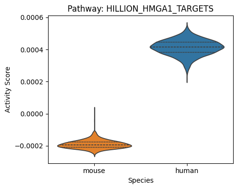
'HILLION_HMGA1_TARGETS': ['CRIP2', 'EDNRB','HSPD1','INSR','GPX3','CXCR4','PMP22','TIMP2','ID2','ID3','MGST1','CD3G','ID1','HSPB1','TFRC','CLU']}
adata = adata_m.concatenate(
adata_h,
batch_key="species",
batch_categories=["mouse", "human"]
)
for key, pathway in pathways.items():
sc.tl.score_genes(adata, gene_list=pathway, score_name=key)
adata_plot = adata[adata.obs.cell_type_fine == plot_cell_type]
fig, ax = plt.subplots(figsize=(5, 4))
sns.violinplot(
data=adata_plot.obs,
x='species',
y=key,
hue='species',
palette={'mouse':'C1','human':'C0'},
dodge=False,
inner='quartile',
ax=ax
)
ax.set_title(f'Pathway: {key}', fontsize=12)
ax.set_xlabel('Species')
ax.set_ylabel('Activity Score')
plt.tight_layout()
plt.show()
/Users/cschaech/Desktop/package_test/.venv/lib/python3.11/site-packages/anndata/_core/anndata.py:1756: UserWarning: Observation names are not unique. To make them unique, call `.obs_names_make_unique`.
  utils.warn_names_duplicates("obs")
/Users/cschaech/Desktop/package_test/.venv/lib/python3.11/site-packages/anndata/_core/anndata.py:1756: UserWarning: Observation names are not unique. To make them unique, call `.obs_names_make_unique`.
  utils.warn_names_duplicates("obs")
/var/folders/bq/cdql_9s11db1zmbxmw_gz7vw0000gn/T/ipykernel_29906/3190824418.py:21: FutureWarning: Use anndata.concat instead of AnnData.concatenate, AnnData.concatenate is deprecated and will be removed in the future. See the tutorial for concat at: https://anndata.readthedocs.io/en/latest/concatenation.html
  adata = adata_m.concatenate(
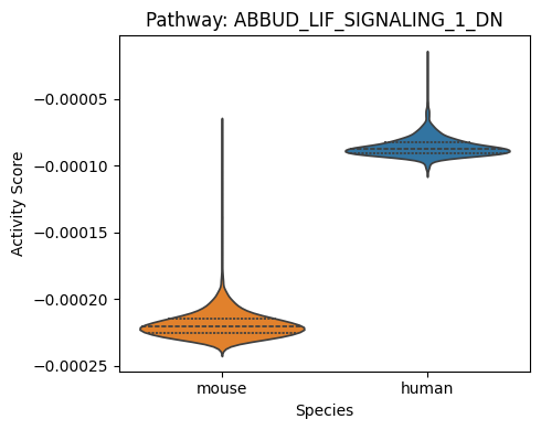
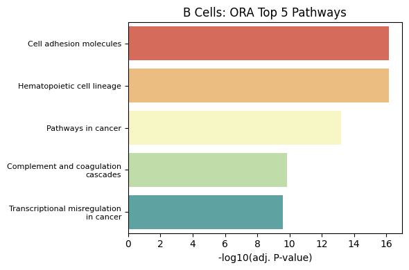
Next we use the differentally expressed genes to analyze pathways. As an example we can create ORA Barplots.
Y-axis: Lists the top five enriched pathways whose member genes are over-represented among the differentially expressed genes.
X-axis (adj. P-value): Longer bars mean more significant enrichment.
[ ]:
import gseapy as gp
import matplotlib.pyplot as plt
import seaborn as sns
import textwrap

cell_type = 'B Cells'
ORA_LIBS = ['KEGG_2021_Human', 'Reactome_Pathways_2024']

df = lfc_dict[cell_type]
degs = df[(df['lfc'].abs() > 1) & (df['p'] > 0.9)]

enr = gp.enrichr(
    gene_list=degs.index.tolist(),
    gene_sets=ORA_LIBS,
    organism='Human',
    outdir=None
)
top5 = enr.results[['Term','Adjusted P-value']].head(5)

wrapped = ["\n".join(textwrap.wrap(t, width=30))
for t in top5['Term']]

fig, ax = plt.subplots(figsize=(6, 4))
sns.barplot(
    x = -np.log10(top5['Adjusted P-value']),
    y = wrapped,
    hue     = wrapped,
    palette = 'Spectral',
    dodge   = False,
    ax = ax
)

ax.set_title(f'{cell_type}: ORA Top 5 Pathways', fontsize=12)
ax.set_xlabel('-log10(adj. P-value)', fontsize=10)
ax.tick_params(axis='y', labelsize=8)
ax.tick_params(axis='x', labelsize=10)
ax.set_ylabel('')

plt.tight_layout()
plt.show()
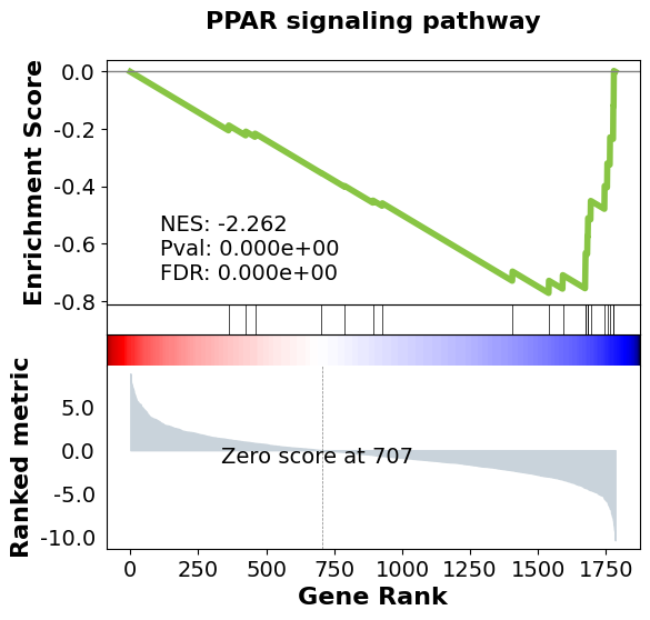
We can also plot the GSEA enrichment curves. We plt the pathway that is the most significant hit by FDR.
X-axis (Rank positions): Genes sorted from highest to lowest log-fold change.
Running Enrichment Score: Curve rises when a pathway gene is encountered and falls otherwise; the peak ES indicates where pathway members cluster in the ranked list.
[ ]:
from gseapy.plot import gseaplot

GSEA_LIB = 'KEGG_2021_Human'

pre_res = gp.prerank(
    rnk            = df['lfc'].sort_values(ascending=False),
    gene_sets      = GSEA_LIB,
    processes      = 4,
    permutation_num=100,
    outdir         = None
)

res = pre_res.res2d.sort_values('FDR q-val')
top_term = res.loc[0, 'Term']
rd = pre_res.results[top_term]

ax = gseaplot(
    term        = top_term,
    hits        = rd['hits'],
    nes         = rd['nes'],
    pval        = rd['pval'],
    fdr         = rd['fdr'],
    RES         = rd['RES'],
    rank_metric = pre_res.ranking,
)
/var/folders/bq/cdql_9s11db1zmbxmw_gz7vw0000gn/T/ipykernel_6592/596071678.py:5: DeprecationWarning: processes is deprecated; use threads
  pre_res = gp.prerank(
4) Creating a cell atlas
NOTE: For differential gene expression analysis the context decoder should be retrained.
[ ]:
model_hamster = scSpecies(device,
                mdata,
                path,
                context_key = 'mouse',
                target_key = 'hamster',
                )

model_hamster.load('context', save_key='_mouse')

model_hamster.train_target(25, save_key='_hamster')
model_hamster.get_representation(eval_model='target', save_libsize=True)
Initializing context scVI model.
Initializing target scVI model.
Loaded /Users/cschaech/Desktop/scpecies_package/scspecies/tutorials/params/config_dict.pkl
Loaded /Users/cschaech/Desktop/scpecies_package/scspecies/tutorials/params/context_config__mouse.pkl
Loaded /Users/cschaech/Desktop/scpecies_package/scspecies/tutorials/params/context_optimizer__mouse.opt
Loaded /Users/cschaech/Desktop/scpecies_package/scspecies/tutorials/params/context_encoder_outer__mouse.pth
Loaded /Users/cschaech/Desktop/scpecies_package/scspecies/tutorials/params/context_decoder__mouse.pth
Loaded /Users/cschaech/Desktop/scpecies_package/scspecies/tutorials/params/target_encoder_inner__mouse.pth
Loaded /Users/cschaech/Desktop/scpecies_package/scspecies/tutorials/params/context_lib_encoder__mouse.pth
Training on the target dataset for 25 epochs (= 1150 iterations).
Progress: 99.4% - ETA: 0:00:00 - Epoch: 25 - Iteration: 1143 - ms/Iteration: 38.25 - nELBO: 1747.0 (+9.752) - nlog_likeli: 1255.4 (+2.519) - KL-Div z: 14.758 (-0.006) - KL-Div l: 2.7907 (+0.007) - Align-Term: 474.04 (+7.233).           Saved /Users/cschaech/Desktop/scpecies_package/scspecies/tutorials/params/config_dict.pkl
Saved /Users/cschaech/Desktop/scpecies_package/scspecies/tutorials/params/target_config__hamster.pkl
Saved /Users/cschaech/Desktop/scpecies_package/scspecies/tutorials/params/target_optimizer__hamster.opt
Saved /Users/cschaech/Desktop/scpecies_package/scspecies/tutorials/params/target_encoder_inner__hamster.pth.
Saved /Users/cschaech/Desktop/scpecies_package/scspecies/tutorials/params/target_encoder_outer__hamster.pth.
Saved /Users/cschaech/Desktop/scpecies_package/scspecies/tutorials/params/target_decoder__hamster.pth.
Saved /Users/cschaech/Desktop/scpecies_package/scspecies/tutorials/params/target_lib_encoder__hamster.pth.
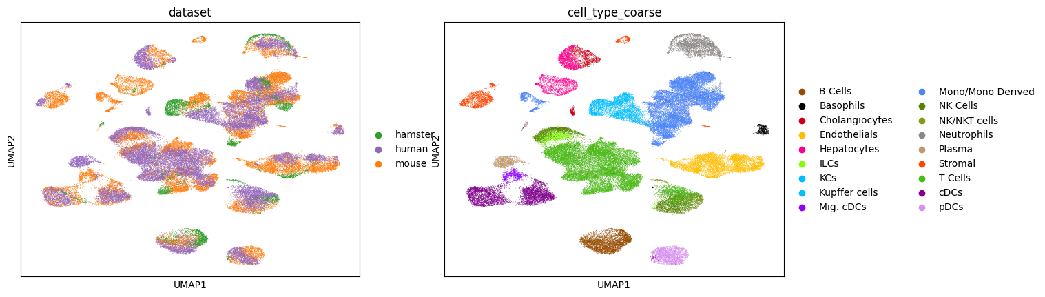
Visualizing the aligned latent space
[ ]:
adata_concat = ad.AnnData(
    X=sparse.vstack([mdata.mod['mouse'].obsm['z_mu'], mdata.mod['human'].obsm['z_mu'], mdata.mod['hamster'].obsm['z_mu']]).toarray(),
    obs=pd.concat([mdata.mod['mouse'].obs[['dataset', 'cell_type_coarse']], mdata.mod['human'].obs[['dataset', 'cell_type_coarse']], mdata.mod['hamster'].obs[['dataset', 'cell_type_coarse']]])
)

# Color scheme for the liver cell dataset. Won't return nice results for other datasets.
palette = return_palette(list(adata_concat.obs.cell_type_coarse.unique()) + list(adata_concat.obs.dataset.unique()))

sc.pp.pca(adata_concat)
neighbors_workaround(adata_concat, use_rep='X_pca')
sc.tl.umap(adata_concat)

sc.pl.umap(adata_concat, color=['dataset', 'cell_type_coarse'], palette=palette)